Restoration of defocused and blurred images
Restoration of distorted images is one of the most interesting and important problems of image processing - from the theoretical, as well as from the practical point of view.
There are especial cases: blurring due to incorrect focus and blurring due to movement - and these very defects (which each of you knows very well, and which are very difficult to repair) were selected as the subject of this article. As for other image defects (noise, incorrect exposure, distortion), the humanity has learned how to correct them, any good photo editor has that tools.
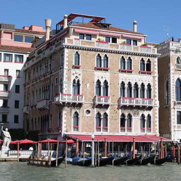
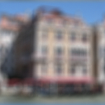
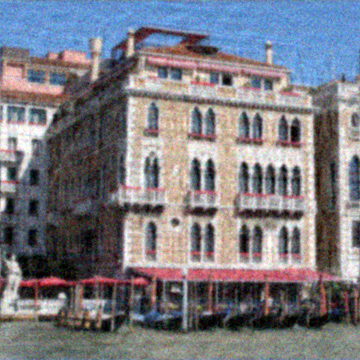
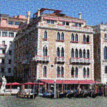
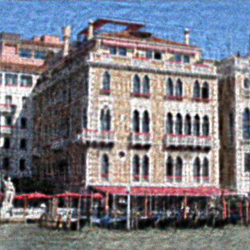
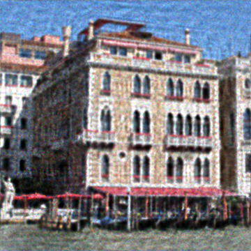
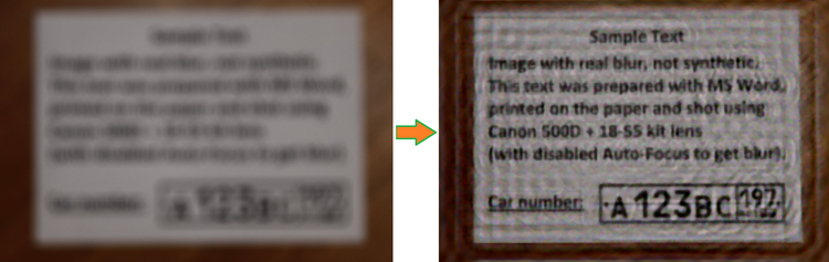
Why is there almost no means for correction of blurring and defocusing (except unsharp mask) - maybe it is impossible to do this at all? In fact, it is possible - development of a respective mathematical theory started approximately 70 years ago, but like other algorithms of image processing, deblurring algorithms became wide-used just recently. So, below is a couple of pictures to demonstrate the WOW-effect:
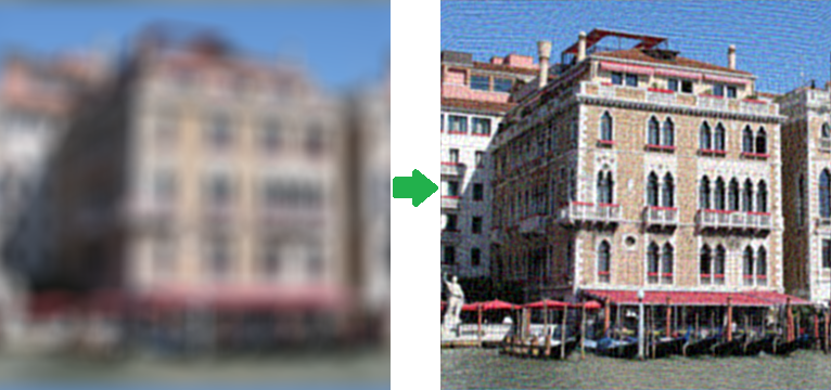
I decided not to use well-known Lena, but just found my own picture of Venice. The right image was really made from the left one, moreover, no optimization like 48-bit format (in this case there will be almost 100% restoration of the source image) were used - there is just a regular PNG with syntetic blur on the left side. The result is impressive... but in practice not everything is so good.
Introduction
Let's start from afar. Many people think that blurring is an irreversible operation and the information in this case is lost for good, because each pixel turns into a spot, everything mixes up, and in case of a big blur radius we will get a flat color all over the image. But it is not quite true - all the information just becomes redistributed in accordance with some rules and can be definitely restored with certain assumptions. An exception is only borders of the image, the width of which is equal to the blur radius - no complete restoration is possible here.
Let's demonstrate it using a small example for a one-dimensional case - let's suppose we have a row of pixels with the
following values:
x1 | x2 | x3 | x4... - Source image
After blurring the value of each pixel is added to the value of the left one: x'i = xi +
xi-1. Normally, it is also required to divide it by 2, but we will drop it out for simplicity. As a result we
have a blurred image with the following pixel values:
x1 + x0 | x2 + x1 | x3 + x2 | x4 +
x3... - Blurred image
Now we will try to restore it, we will consequentially subtract values according to the following scheme - the first pixel
from the second one, the result of the second pixel from the third one, the result of the third pixel from the fourth
one and so on, and we will get the following:
x1 + x0 | x2 - x0 | x3 + x0 | x4 -
x0... - Restored image
As a result, instead of a blurred image, we got the source image with added to the each pixel an unknown constant x0 with the alternate sign. This is much better - we can choose this constant visually, we can suppose that it is approximately equal to the value x1, we can automatically choose it with such a criteria that values of neighboring pixels were changing as little as possible, etc. But everything changes as soon as we add noise (which is always present in real images). In case of the described scheme on each stage there will accumulate the noise value into the total value, which fact eventually can produce an absolutely unacceptable result, but as we already know, restoration is quite possible even using such a primitive method.
Blurring process model
Now let's pass on to more formal and scientific description of these blurring and restoration processes. We will
consider only grayscale images, supposing that for processing of a full-color image it is enough to
repeat all required steps for each of the RGB color channels. Let's introduce the following definitions:
f(x, y) - source image (non-blurred)
h(x, y) - blurring function
n(x, y) - additive noise
g(x, y) - blurring result image
We will form the blurring process model in the following way:
g(x, y) = h(x, y) * f(x, y) + n(x, y) (1)
The task of restoration of a blurred image consists in finding the best approximation f'(x, y) to the source
image. Let's consider each component in a more detailed way. As for functions f(x, y) and g(x, y),
everything is quite clear with them. But as for h(x, y) I need to say a couple of words - what is it? In the
process of blurring the each pixel of a source image turns into a spot in case of defocusing and into a line segment (or some path) in case
of a usual blurring due to movement. Or we can say otherwise, that each pixel of a blurred image is "assembled" from
pixels of some nearby area of a source image. All those overlap each other, which fact results in a blurred image. The
principle, according to which one pixel becomes spread, is called the blurring function. Other synonyms -
PSF (Point spread function), kernel and other. The size of this function is lower than the size of the image
itself - for example, when we were considering the first "demonstrational" example the size of the function was 2,
because each result pixel consisted of two pixels.
Blurring functions
Let us see what typical blurring functions look like. Hereinafter we will use the tool which has already become standard for such purposes - Matlab, it contains everything required for the most diverse experiments with image processing (among other things) and allows to concentrate on algorithms, shifting all the routine work to function libraries. However, this is only possible at the cost of performance. So, let's get back to PSF, here are their examples:
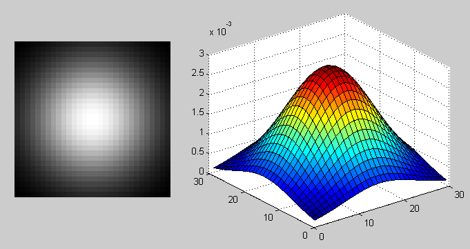
PSF in case of Gaussian functions using: fspecial('gaussian', 30, 8);
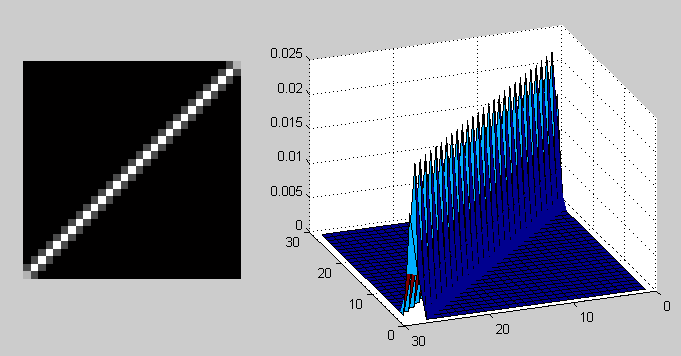
PSF in case of motion blur functions using: fspecial('motion', 40, 45);
The process of applying of the blurring function to another function (in his case, to an image) is called convolution, i.e. some area of the source image convolves into one pixel of the blurred image. It is denoted through the operator "*", but do not confuse it with a simple multiplication! Mathematically, for an image f with dimensions M x N and the blurring function h with dimensions m x n it can be written down as follows:
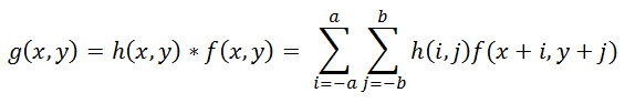 |
(2) |
Where a = (m - 1) / 2, b = (n - 1) / 2. The process, which is opposite to convolution, is called deconvolution and solution of such task is quite uncommon.
Noise model
It is only left to consider the last summand, which is responsible for noise, n(x, y) in the formula (1). There can be many reasons for noise in digital sensors, but the basic ones are - thermal vibrations (Brownian motion) and dark current. The noise volume also depends on a number of factors, such as ISO value, sensor type, pixel size, temperature, magnetic field value, etc. In most cases there is Gaussian noise (which is set by two parameters - the average and dispersion), and it is also additive, does not correlate with an image and does not depend on pixel coordinates. The last three assumptions are very important for further work.
Convolution theorem
Let us get back to the initial task of restoration - we need to somehow reverse the convolution, bearing in mind the noise. From the formula (2) we can see that it is not so easy to get f(x, y) from g(x, y) - if we calculate it straightforward, then we will get a huge set of equations. But the Fourier transform comes to the rescue, we will not view it in details, because a lot has been said about this topic already. So, there is the so called convolution theorem, according to which the operation of convolution in the spatial domain is equivalent to regular multiplication in the frequency domain (where the multiplication - element-by-element, not matrix one). Correspondingly, the operation which is opposite to convolution is equivalent to division in the frequency domain, i.e. this can be expressed as follows:
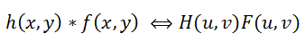 |
(3) |
Where H(u, v), F(u, v) - Fourier functions for h(x,y) and f(x,y). So, the blurring process from (1) can be
written over in the frequency domain as:
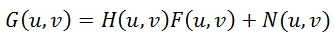 |
(4) |
Inverse filter
Here we are tempted to divide this equation by H(u, v) and get the following evaluation F^(u,
v) of the source image:
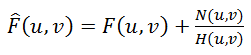 |
(5) |
This is called inverse filtering, but in practice it almost never works. Why so? In order to answer this question, let
us see the last summand in the formula (5) - if the function H(u, v) gives values, which are close to zero or
equal to it, then the input of this summand will be dominating. This can be almost always seen in real examples - to
explain this let's remember what a spectrum looks like after the Fourier transform.
So, we take the source image,
convert it into a grayscale one, using Matlab, and get the spectrum:
% Load image
I = imread('image_src.png');
figure(1); imshow(I); title('Source image');
% Convert image into grayscale
I = rgb2gray(I);
% Compute Fourier Transform and center it
fftRes = fftshift(fft2(I));
% Show result
figure(2); imshow(mat2gray(log(1+abs(fftRes)))); title('FFT - amplitude spectrum (log scale)');
figure(3); imshow(mat2gray(angle(fftRes))); title('FFT - phase smectrum');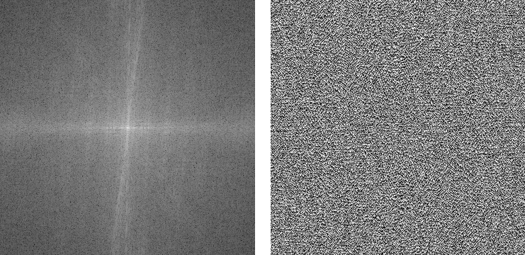
As a result we will have two components: amplitude and phase spectrum. By the way, many people forget about the phase. Please note that the amplitude spectrum is shown in a logarithmic scale, because its values vary tremendously - by several orders of magnitude, in the center the values are maximum (millions) and they quickly decay almost to zero ones as they are getting farther from the center. Due to this very fact inverse filtering will work only in case of zero or almost zero noise values. Let's demonstrate this in practice, using the following script:
% Load image
I = im2double(imread('image_src.png'));
figure(1); imshow(I); title('Source image');
% Blur image
Blurred = imfilter(I, PSF,'circular','conv' );
figure(2); imshow(Blurred); title('Blurred image');
% Add noise
noise_mean = 0;
noise_var = 0.0;
Blurred = imnoise(Blurred, 'gaussian', noise_mean, noise_var);
% Deconvolution
figure(3); imshow(deconvwnr(Blurred, PSF, 0)); title('Result');
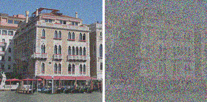
| noise_var = 0.0000001 | noise_var = 0.000005 |
It is well seen that addition of even a very small noise causes serious distortions, which fact substantially limits
application of the method.
Existing approaches to deconvolution
There are approaches, which take into account the presence of noise in an image - one of the most popular and the first
ones, is Wiener filter. It considers the image and the noise as random processes and finds such a value of f' for
a distortion-free image f, that the mean square deviation of these values was minimal. The minimum of such
deviation is achieved at the function in the Frequency domain:
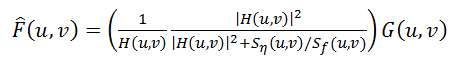 |
(6) |
This result was found by Wiener in 1942. We will not give his detailed conclusion in this article, those interested can find it here. The S function denotes here the energy spectrum of noise and of the source image respectively - as these values are rarely known, then the fraction Sn / Sf is replaced by some constant K, which can be approximately characterized as the signal-noise ratio.
The next method is "Constrained Least Squares Filtering", other names: "Tikhonov filtration", "Tikhonov regularization".
His idea consists in formation of a task in the form of a matrix with subsequent solution of the respective optimization
task. This equation result can be written down as follows:
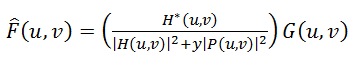 |
(7) |
Where y - regularization parameter, а P(u, v) - Fourier-function of Laplace operator (matrix 3 * 3).
Another interesting approach was offered by Richardson (1972 year) and Lucy independently (1974 year), so this approach
is called as method Lucy-Richardson. Its distinctive feature consists in the fact that it is nonlinear, unlike the first
three - potentially this can give a better result. The second feature - this method is iterative, so there arise
difficulties with the criterion of iterations stop. The main idea consists in using the maximum likelihood method for
which it is supposed that an image is subjected to Poisson distribution. Calculation formulas are quite simple, without
the use of Fourier transform - everything is done in the spatial domain:
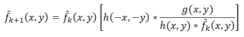 |
(8) |
Here the symbol "*", as before, denotes the convolution operation. This method is widely used in programs for processing of astronomical photographs - use of deconvolution in them (instead of unsharp mask, as in photo editors) is a de-facto standard. Computational complexity of the method is quite high - processing of an average photograph, depending on the number of iterations, can take many hours and even days.
The last considered method, or to be exact, the whole family of methods, which are no being actively developed - is blind deconvolution. In all previous methods it was supposed that the blurring function PSF is known for sure, but in practice it is not true, usually we know just the approximate PSF by the type of visible distortions. Blind deconvolution is the very attempt to take this into account. The principle is quite simple, without going deep into details - there is selected the first approximation of PSF, then deconvolution is performed using one of the methods, following which the degree of quality is identified according to some criterion, based on this degree the PSF function is tuned and iteration repeats until the required result is achieved.
Practice
Now we are don with the theory - let's pass on to practice, we will start with comparison of listed methods on an image
with syntetic blur and noise.
% Load image
I = im2double(imread('image_src.png'));
figure(1); imshow(I); title('Source image');

% Blur image
PSF = fspecial('disk', 15);
Blurred = imfilter(I, PSF,'circular','conv' );

% Add noise
noise_mean = 0;
noise_var = 0.00001;
Blurred = imnoise(Blurred, 'gaussian', noise_mean, noise_var);
figure(2); imshow(Blurred); title('Blurred image');
estimated_nsr = noise_var / var(Blurred(:));

% Restore image
figure(3), imshow(deconvwnr(Blurred, PSF, estimated_nsr)), title('Wiener');
figure(4); imshow(deconvreg(Blurred, PSF)); title('Regul');
figure(5); imshow(deconvblind(Blurred, PSF, 100));
title('Blind');
figure(6); imshow(deconvlucy(Blurred, PSF, 100));
title('Lucy');
Results:
 |
 |
| Wiener filter | Tikhonov regularization |
 |
 |
| Lucy-Richardson filter | Blind deconvolution |
Conclusion
And at the end of the first part we will consider examples of real images. Before that all blurs were artificial, which is quite good for practice and learning, but it is very interesting to see how all this will work with real photos. Here is one example of such image, shot with the Canon 500D camera using manual focus (to get blur):
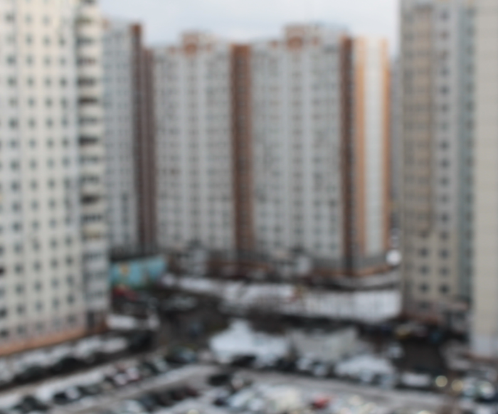
Then we run the script:
% Load image
I = im2double(imread('IMG_REAL.PNG'));
figure(1); imshow(I); title('Source image');

%PSF
PSF = fspecial('disk', 8);
noise_mean = 0;
noise_var = 0.0001;
estimated_nsr = noise_var / var(I(:));

I = edgetaper(I, PSF);
figure(2); imshow(deconvwnr(I, PSF, estimated_nsr)); title('Result');
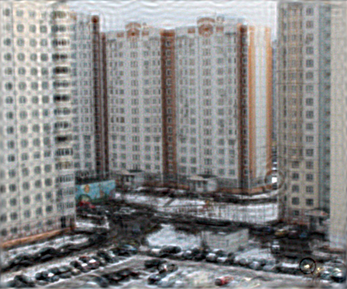
As we can see, new details appeared on the image, sharpness became much higher, however there appeared "ring effect" on the sharp borders.
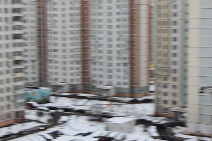
And an example with a real blur due to movement - in order to make this the camera was fixed on a tripod, there was set
quite long exposure value and with an even movement at the moment of exposure the following blur was obtained:
The script is almost the same, but the PSF type is "motion":
% Load image
I = im2double(imread('IMG_REAL_motion_blur.PNG'));
figure(1); imshow(I); title('Source image');

%PSF
PSF = fspecial('motion', 14, 0);
noise_mean = 0;
noise_var = 0.0001;
estimated_nsr = noise_var / var(I(:));

I = edgetaper(I, PSF);
figure(2); imshow(deconvwnr(I, PSF, estimated_nsr)); title('Result');
Result:
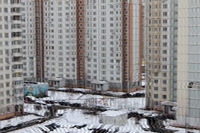
Again the quality noticeably increased - window frames, cars became recognizable. Artifacts are now different, unlike in
the previous example with defocusing.
Practical implementation. SmartDeblur
I created a program, which demonstrates restoration of blurred and defocused images. Written on C++ using Qt. I
chose the FFTW library, as the fastest open source implementations of Fourier transform.
My program is called SmartDeblur, windows-binaries and sources you can from GitHub:
https://github.com/Y-Vladimir/SmartDeblur/downloads
All source files are under the GPL v3 license.
Screenshot of the main window:

Main functions:
- High speed. Processing of an image with the size of 2048*1500 pixels takes about 300ms in the Preview mode (when adjustment sliders can move). But high-quality processing may take a few minutes
- Real-time parameters changes applying (without any preview button)
- Full resolution processing (without small preview window)
- Deep tuning of kernel parameters
- Easy and friendly user interface
- Help screen with image example
- Deconvolution methods: Wiener, Tikhonov, Total Variation prior
And in the conclusion let me demonstrate one more example with real (not syntetic) out-of-focus blur:
That's all for the first part.
In the second part I will focus on problems with real images processing - creation of PSF and their evaluation, will
introduce more complex and advanced deconvolution techniques, methods of ring effect elimination, will make a review of
existing deconvolution software and compare it.
If you have any questions please contact me by email - I will be happy if you give me any feedback regarding this
article and SmartDeblur.
 (Vladimir Yuzhikov)
P.S. Russian translate can be found here
See continue here
(Part II - practical issues and their solutions, blind deconvolution)
Social links
Discussion on Reddit
Discussion on Gizmodo
Discussion on Hacker News
| Tweet |